Disney BSDF
Relevant code:
src/disney.cppinclude/nori/warp.hsrc/warp.cppsrc/warptest.cpp
For my first advanced feature, I chose to implement Disney's Principled
BSDF. This is a key feature that that can model
a wide variety of surfaces, essentially working as a single BSDF
that can be used for every object in a scene.
This feature has a variety of intuitive parameters that work
to create a robust set of surface models rather than be perfectly physically correct.
This BSDF also supports image textures for the albedo, as well as bump mapping.
In order to use the BSDF, you can include the following inside a mesh in the scene file:
Example Usage:
                        <bsdf type="disney">

                        <color name="baseColor" value="1.0, 0.0, 0.0"/>

                        <float name="metallic" value="0.0"/>

                        <float name="specular" value="0.0"/>

                        <float name="specularTint" value="0.0"/>

                        <float name="roughness" value="0.0"/>

                        <float name="clearcoat" value="0.0"/>

                        <float name="clearcoatGloss" value="0.0"/>

                        <bsdf/>
Note that all the parameters are meant to be in the range \([0, 1]\). Additionally,
they each have defaults so you only need to include the parameters you would like
to change in the scene description.
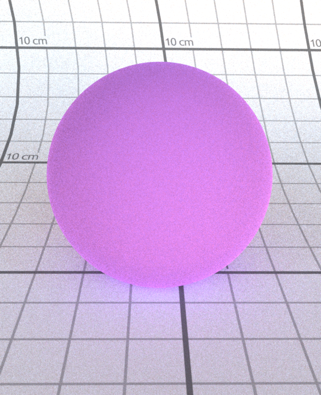
Validation and Implementation:
All following images are the results from rendering analytical spheres with an
EnvMap Emitter on both Nori and Mitsuba. For each section, all
parameters are held at some constant value (may not be default) while the defined
parameter varies. The code
for these scenes can be found in scenes/val/disney/*/*.xml
and scenes/mitsuba/disney/*/*.xml
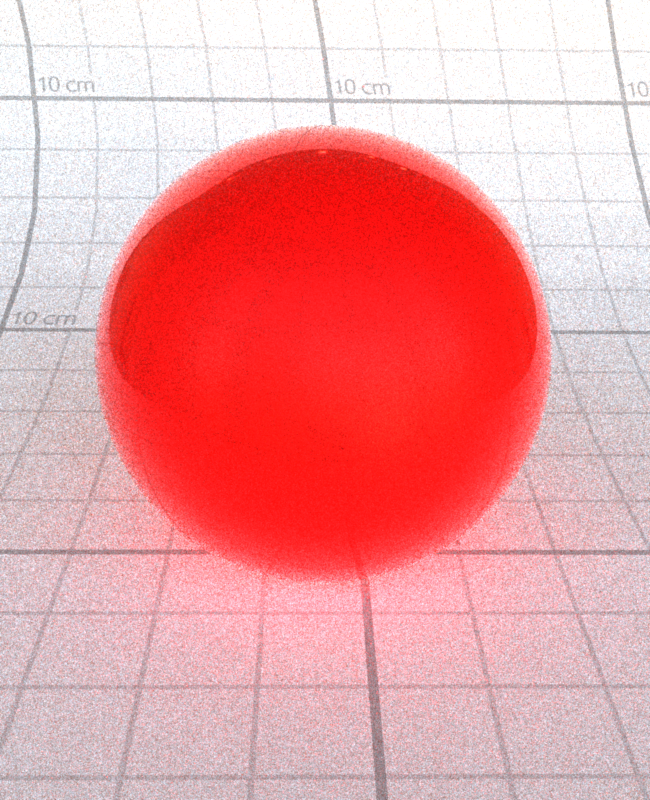
Base Color:
My implementation of the Disney BSDF is made up of three lobes:
- Diffuse
- Specular
- Clearcoat
baseColor parameter contributes to both the Diffuse and Specular lobes.
We will first begin by looking at the diffuse, which uses a Schlick Fresnel
approximation and modifies the grazing retroreflection response to get a specific value
determined from roughness. The model is as follows:
\[ f_d = \frac{baseColor}{\pi} (1 + (F_{D90} - 1) (1 - \cos \theta_l)^5) (1 + (F_{D90} - 1) (1 - \cos \theta_v)^5) \]
where
\[ F_{D90} = 0.5 + 2roughness\cos^2{\theta_d} \]
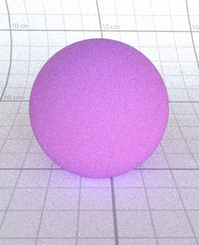
Overall, this parameter is the most fundamental and produces the largest difference as we let it vary:
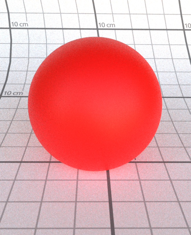
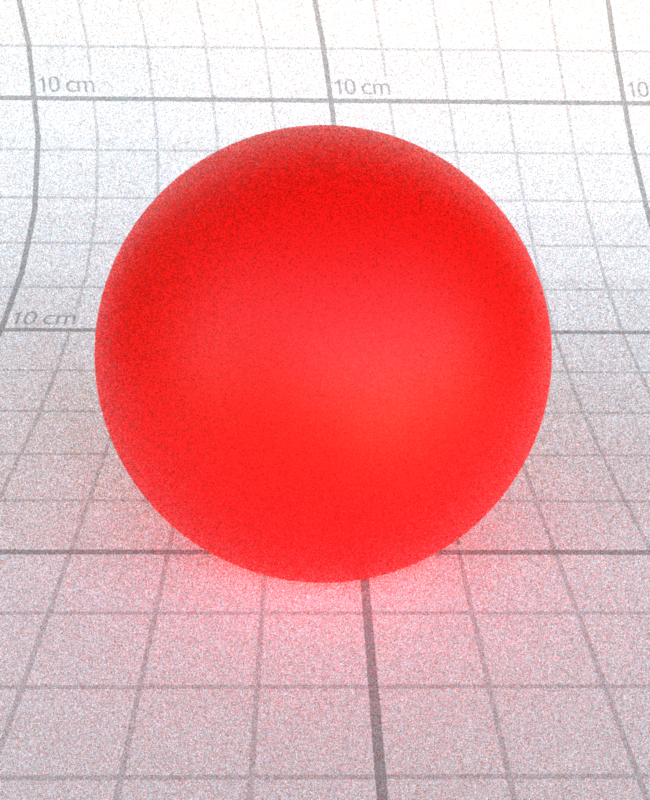
\[baseColor = 1.0, 0.0, 0.0\]

\[baseColor = 1.0, 0.5, 0.0\]


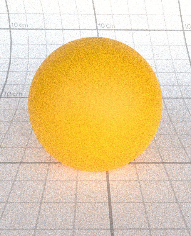
\[baseColor = 1.0, 1.0, 0.0\]


\[baseColor = 0.0, 0.5, 0.0\]

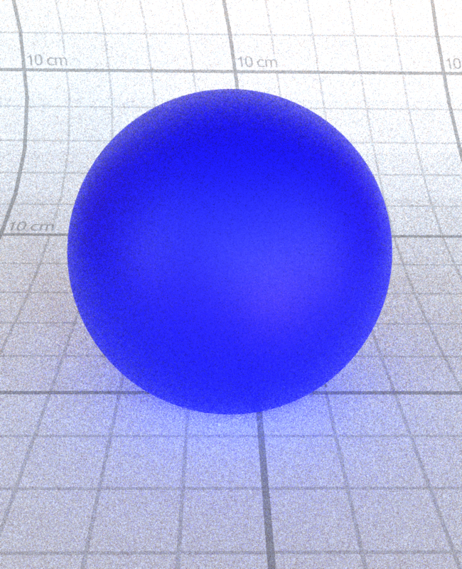
\[baseColor = 0.0, 0.0, 1.0\]
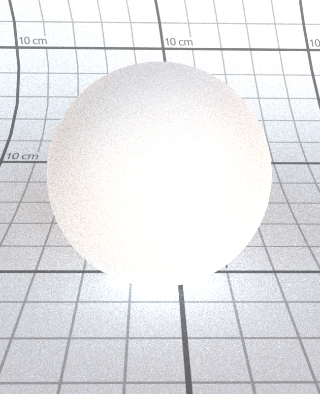

\[baseColor = 1.0, 1.0, 1.0\]
Specular:
Next, the Specular Lobe is implemented using a standard microfacet model defined by:
\[ f_s(\theta_i, \theta_o) = \frac{F(\theta_i)D(\theta_h)G(\theta_i,\theta_o)}{4\cos\theta_i\cos\theta_o} \]
In this case, \(F\) is again a Schlick Fresnel approximation of a mix of metallic, specular,
baseColor and specularTint parameters. \( D \) is the normal distribution using the
Generalized-Trowbridge-Reitz (GTR) distribution:
\[ D_{GTR}(\theta_h) = \frac{c}{(\alpha^2 \cos^2\theta_h + \sin^2\theta_h)^\gamma} \]
where \( c \) is a normalization constant and \( \alpha \) is the roughness value. For this case
in particular, we use the GTR2 distribution with \( \gamma = 2 \) and \( \alpha = roughness^2 \).
Finally, the shadowing term \( G \) is modeled by the Smith GGX Distribution. Disney's implementation
also includes some remapping of parameters to be more "artistically pleasing". While my implementation
follows the distribution, I have not completely remapped the parameters, leading to a slightly different
results.
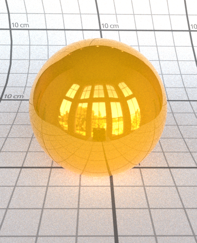
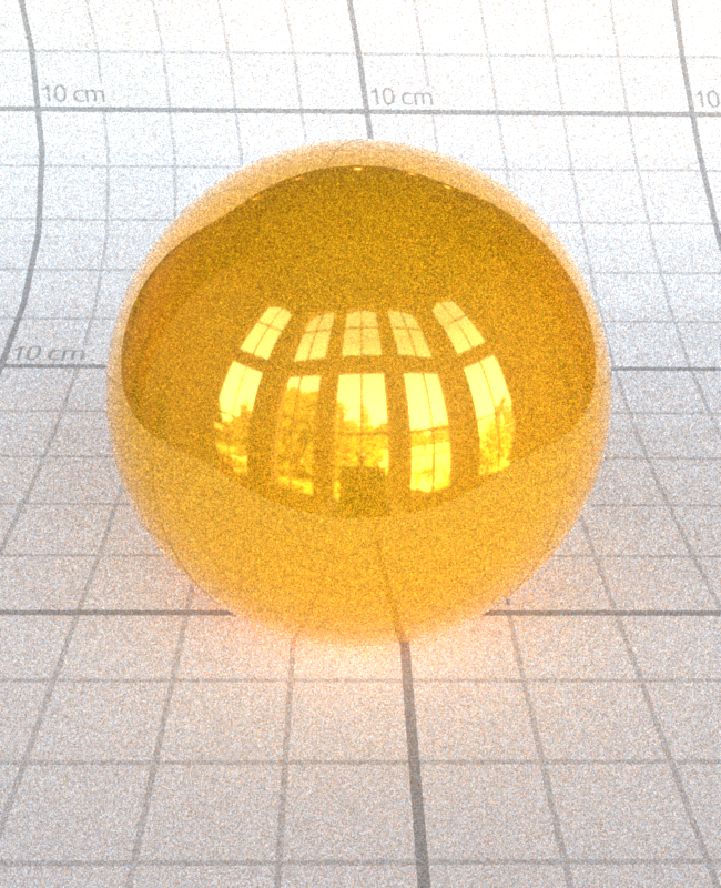
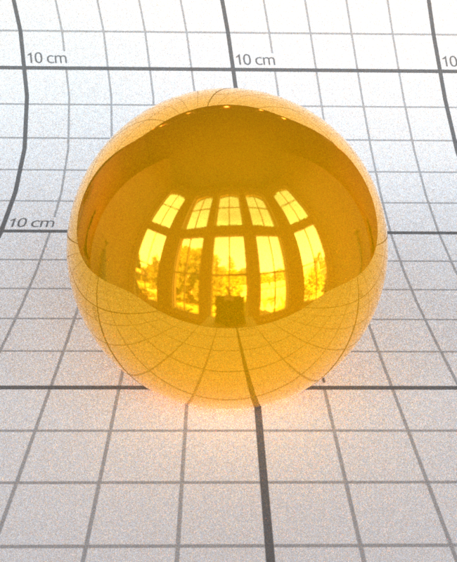
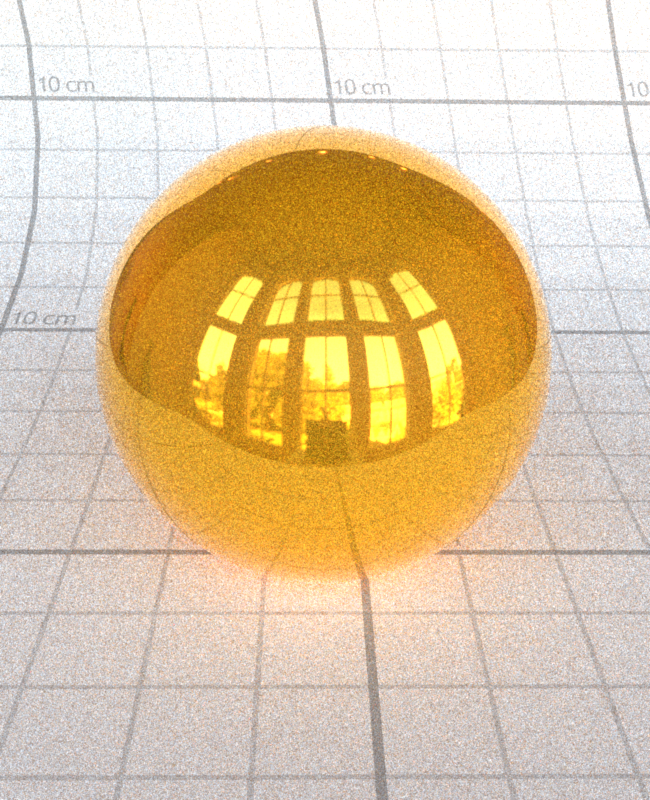
Overall, this model produces intuitive results, increasing the reflectiveness, or specularity,
as the parameter increases:
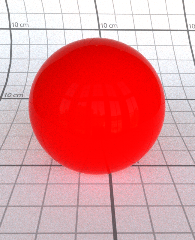
\[specular = 0.0\]

\[specular = 0.2\]

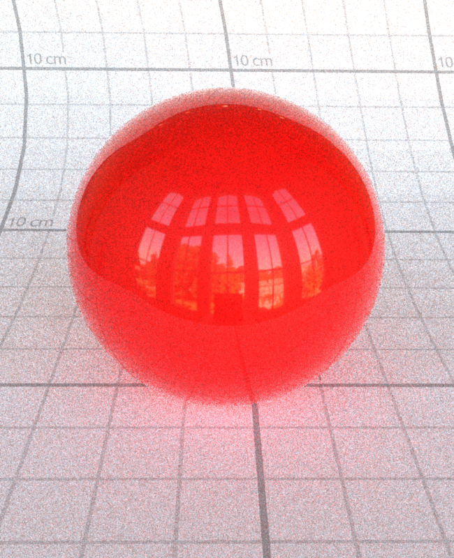
\[specular = 0.4\]
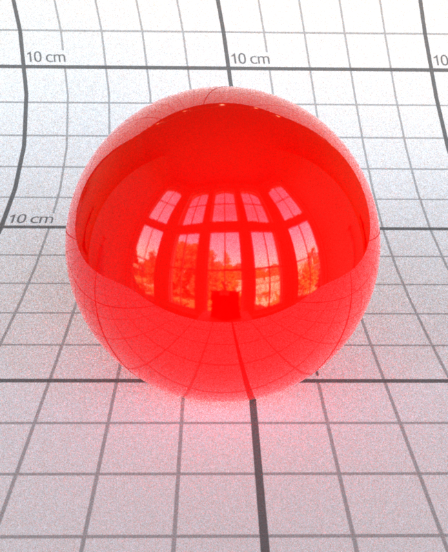
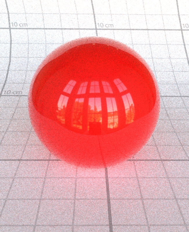
\[specular = 0.6\]
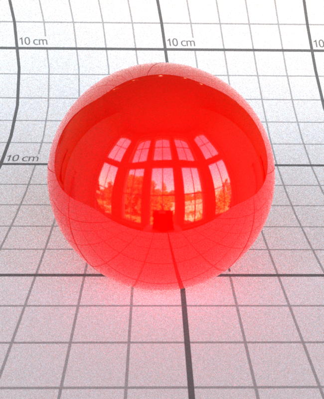

\[specular = 0.8\]


\[specular = 1.0\]
Specular Tint:
As mentioned above, the specularTint parameter is used
in the Fresnel Approximation of the Specular Lobe. It is linearly interpolated
with the color of the tint calculated with the baseColor and
a linearly remapped specular parameter. As you can see below,
the color of the reflection leans further towards the base color as the parameter
increases.


\[specularTint = 0.0\]

\[specularTint = 0.2\]

\[specularTint = 0.4\]


\[specularTint = 0.6\]
\[specularTint = 0.8\]

\[specularTint = 1.0\]
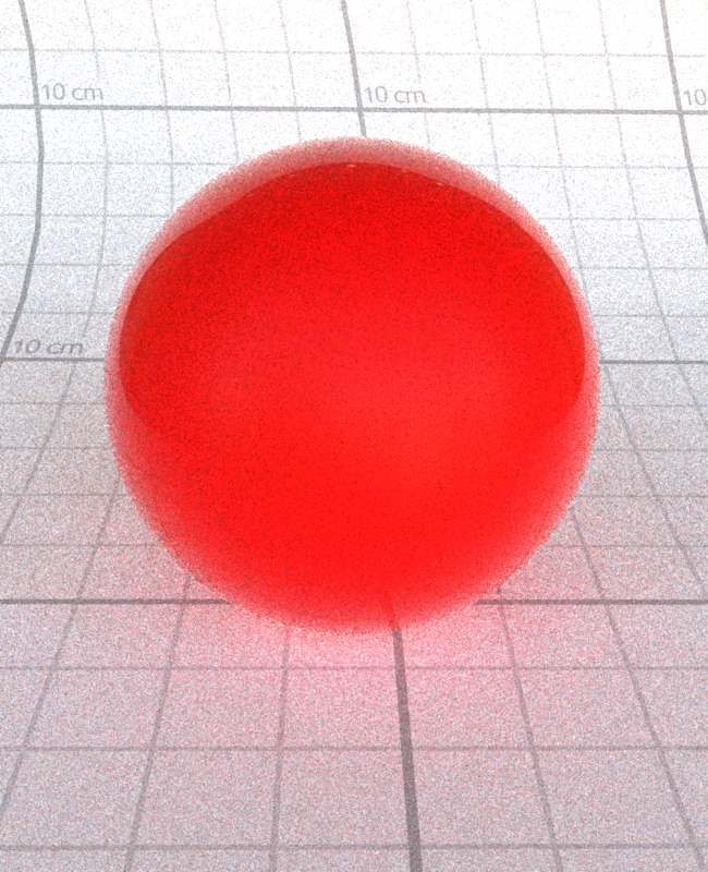
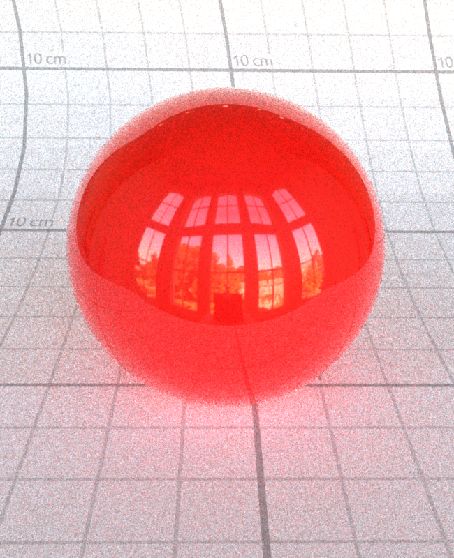
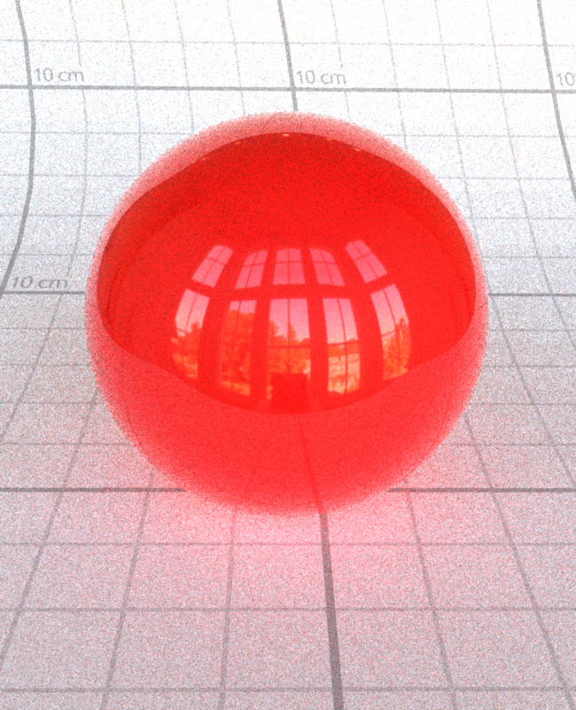
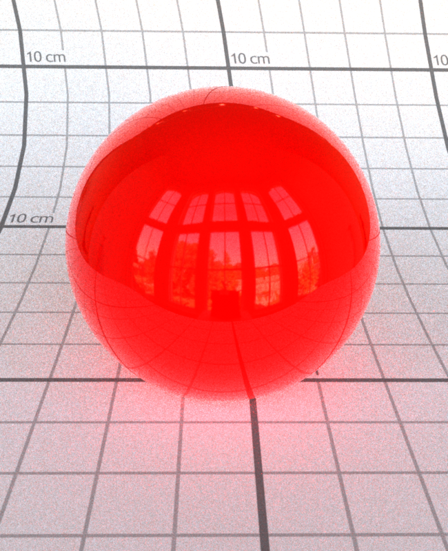
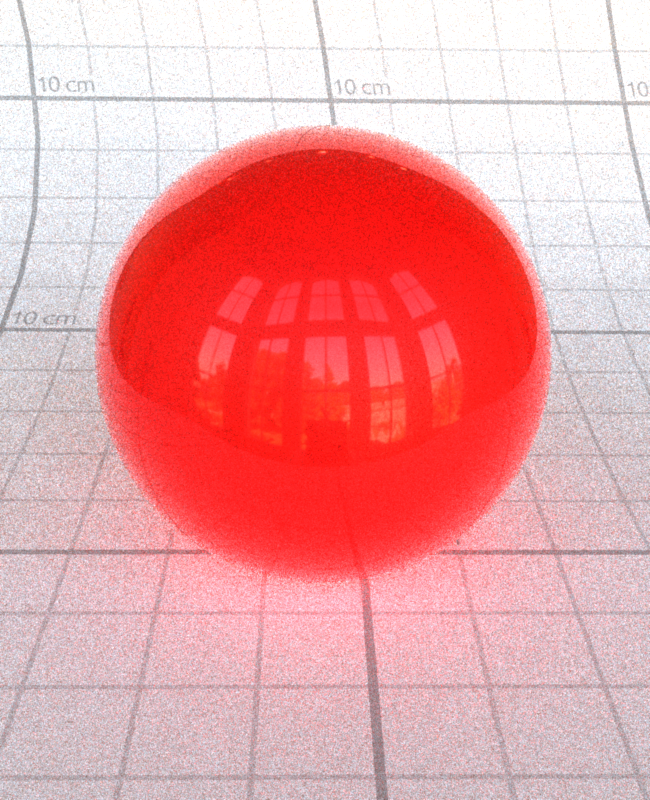
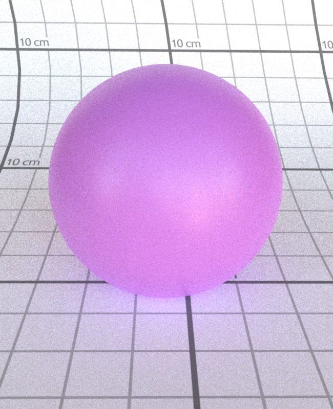
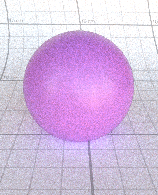
Roughness:
As also mentioned above, the roughness contributes to both the
grazing retroreflection response in the Diffuse Lobe, and the \(\alpha\) term
in the GTR2 and Smith GGX distributions. With an effect on both lobes, it is
clearly able to decrease the reflectance of the surface as it is increased:

\[roughness = 0.0\]


\[roughness = 0.2\]
\[roughness = 0.4\]


\[roughness = 0.6\]


\[roughness = 0.8\]
\[roughness = 1.0\]
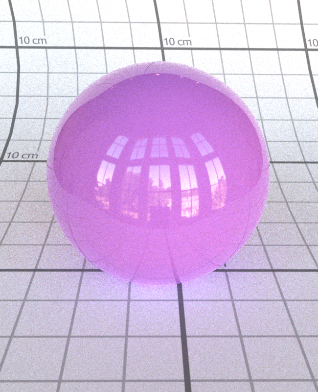
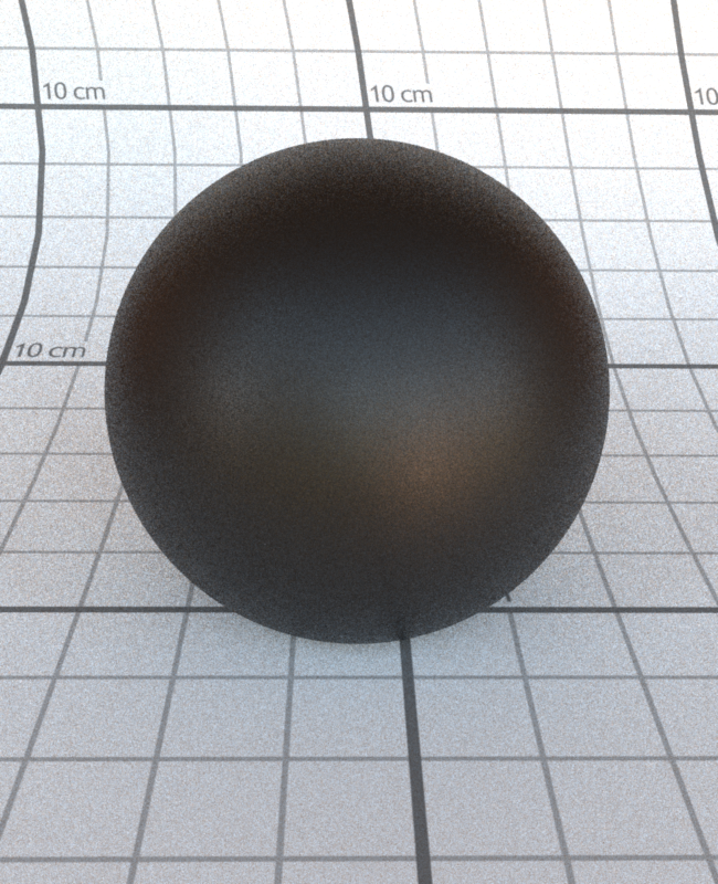
Metallic:
The metallic parameter contributes to both the Diffuse Lobe
and the Specular Lobe, working to effectively scale and balance how
much the Diffuse Lobe is contributing. In my evaluation of the Disney BSDF,
my returned value is:
\[ f_{disney} = (1 - metallic) * f_{diffuse} + f_{specular} + clearcoat * f_{clearcoat} \]
This means that as the metallic parameter approaches 1, only the
Specular and Clearcoat lobes will contribute, leading to a large amount of reflection.


\[metallic = 0.0\]
\[metallic = 0.2\]
\[metallic = 0.4\]
\[metallic = 0.6\]
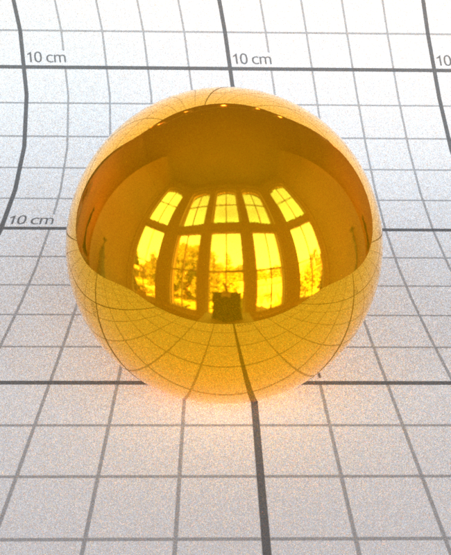
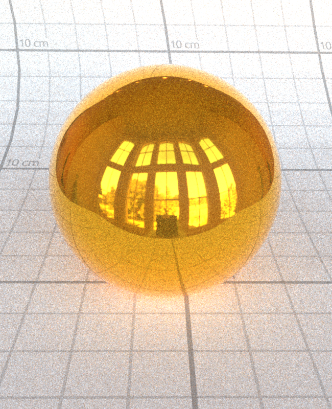
\[metallic = 0.8\]

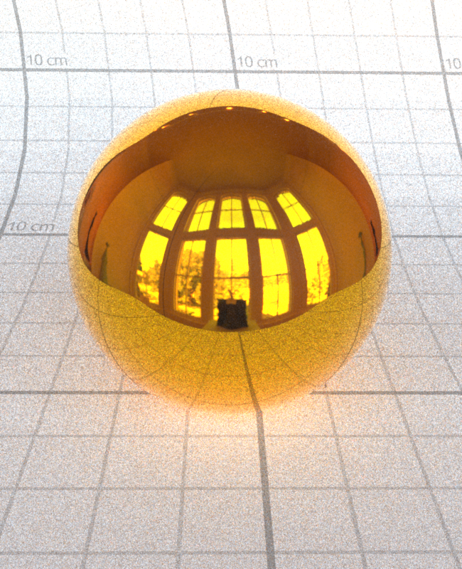
\[metallic = 1.0\]
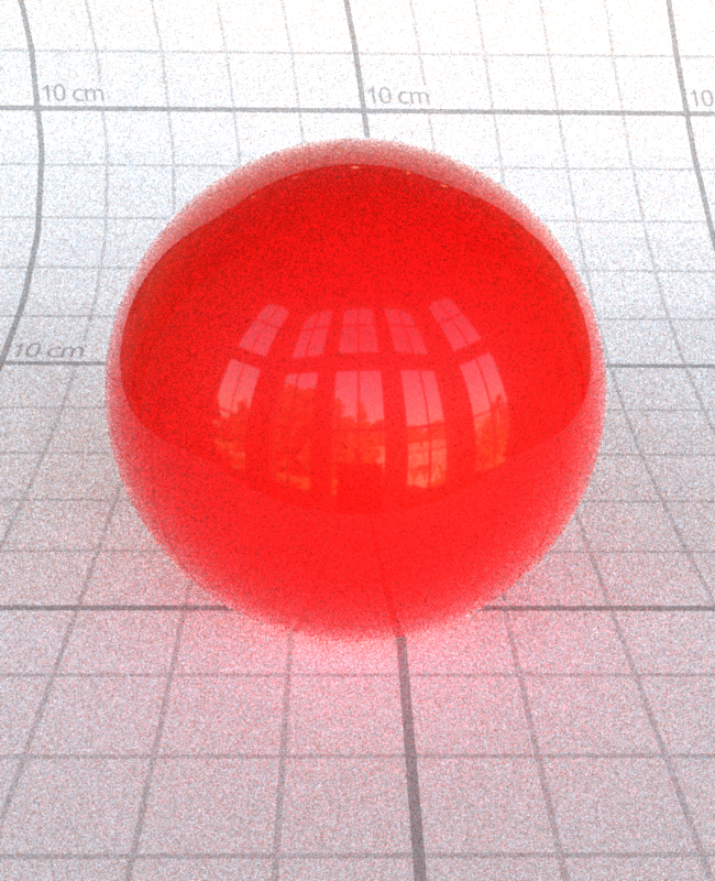
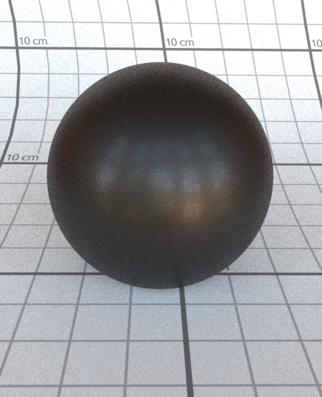
Clearcoat:
Lastly, the Clearcoat Lobe is also implemented using a standard microfacet model defined by:
\[ f_s(\theta_i, \theta_o) = \frac{F(\theta_i)D(\theta_h)G(\theta_i,\theta_o)}{4\cos\theta_i\cos\theta_o} \]
In this case, \(F\) is Schlick Fresnel approximation with a fixed IOR of \(1.5\). \( D \) is again the normal distribution using the
Generalized-Trowbridge-Reitz (GTR) distribution but in this case the GTR1 distribution with
\( \gamma = 1 \) and \( \alpha \) a linear interpolation of the clearcoatGloss parameter.
The shadowing term \( G \) is also modeled by the Smith GGX Distribution, but now with a roughness value fixed at \(0.25\).
Note that again, this doesn't take the exact same approach as Disney's remapped implementation, resulting in slightly
different results.
Overall, while slightly different than Mitsuba, the desired effect is still found whereby increasing the clearcoat subtly
increases the reflection on the surface as a thin clear layer.

\[clearcoat = 0.0\]

\[clearcoat = 0.2\]

\[clearcoat = 0.4\]
\[clearcoat = 0.6\]

\[clearcoat = 0.8\]
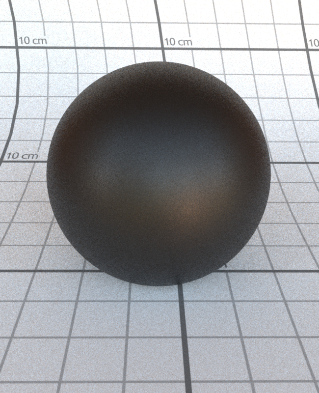
\[clearcoat = 1.0\]
Clearcoat Gloss:
As mentioned above, the clearcoatGloss parameter is used
in the GTR1 Distribution of the Clearcoat Lobe. It is linearly interpolated
with some constants, working to produce the "glossiness" of the Lobe. As you can see below,
the reflection of the Clearcoat Lobe becomes more intense as the parameter increases.

\[clearcoatGloss = 0.0\]

\[clearcoatGloss = 0.2\]

\[clearcoatGloss = 0.4\]

\[clearcoatGloss = 0.6\]
\[clearcoatGloss = 0.8\]

\[clearcoatGloss = 1.0\]
Importance Sampling:
In order to sample from the Disney BRDF, I effectively assign weights to each Lobe,
take a random sample, and then based on the weights directly sample one of the lobes.
I begin by assigning a weight of
\[ diffuseWeight = \frac{1 - metallic}{2} \]
Then, if the uniform sample is less than this value, I simply sample from
a Cosine-Weighted Hemisphere. If not, I rescale the point to be uniform, and then
assign a weight
\[ specularWeight = \frac{1}{1 + clearcoat} \]
to the Specular Lobe. If the newly scaled sample is less than this, I simply
sample from the GTR2 distribution. Finally, if I still have not sampled, I
default to the Clearcoat Lobe and will take a sample from the GTR1 distribution.
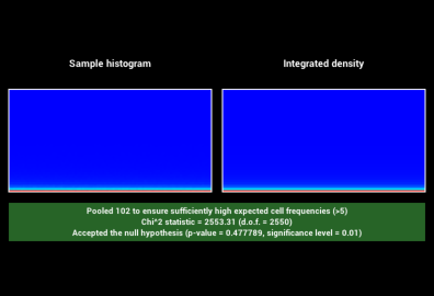
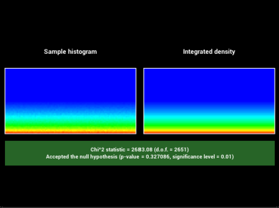
In order to verify that my new sampling methods GTR1 and GTR2 are valid, I
added code to warptest.cpp to ensure the sampling methods were correct:
GTR1 Sampling Validation:

\[\alpha = 0.05\]
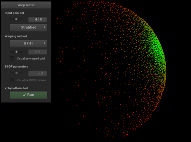
\[\alpha = 0.2\]
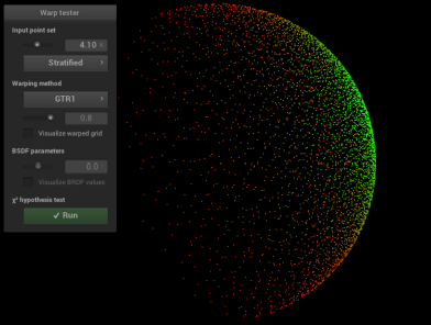
\[\alpha = 0.8\]
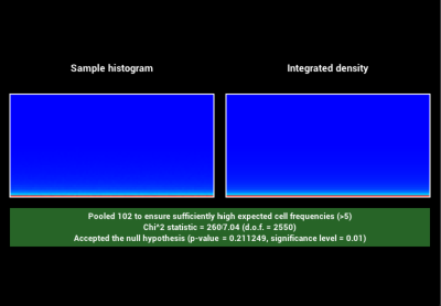


GTR2 Sampling Validation:
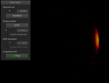
\[\alpha = 0.05\]
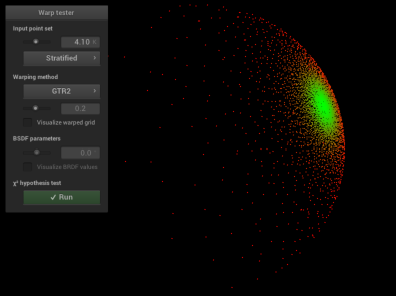
\[\alpha = 0.2\]
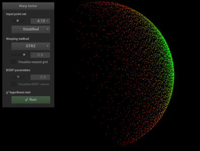
\[\alpha = 0.8\]

Problems and External Libraries:
This feature required significantly more work and time than any of the basic features, but
overall went pretty smoothly with the large amount of documentation and examples.
Specifically, I found the
Physically Based Shading at Disney
paper as well as the
Official Disney BRDF Implementation particularly
helpful. They contained all of the theory behind the models used, as well as an example
of the implementation for some of the functions. With this, no external libraries were required as I was able to implement
the required distribution functions myself in both src/disney.cpp and src/warp.cpp.
Environment Map Emitter
Relevant code:
src/envmap.cpp
For my second advanced feature, I chose to implement Environment Mapping.
Essentially, this is an infinite area light that can be through of as
an enormous sphere that casts light in to the scene from all directions.
The input to the scene is a HDRI environment map parameterized by longitude \(\theta\)
and latitude \(\phi\). It can very simply be added to the scene with the following:
Example Usage:
                        <mesh type="sphere">

                        ...

                        <emitter type="envmap">

                        <string name="filename" value="envmap.exr" />
</emitter>
</mesh>
Implementation:
The implementation of this feature begins relatively similar to ImageTextures. The class
first reads in the file and stores it as a matrix of Color3f. However, in this
case, it reads the Bitmap pixel-by-pixel and stores the luminance value at each point. This
is where the similarities to Image Textures end. We will
then treat this matrix as a piecewise constant 2D function \(f\) with inputs \(u, v\) (not yet \(\theta, \phi\)).
In order to effectively draw samples
from this map, we work to precompute the Marginal PDF and CDF and the Conditional PDF and CDF that can
later be quickly and efficiently importance sampled. The process looks like the following:
First, in the constructor of EnvMap precompute2D() is called. This function
iterates over all \(u\) values in the image, considering one row of the matrix at a time.
For each row, it then computes the 1-dimensional PDF and CDF for the row, which is just the conditional
PDF \(p_v(v | u) = \frac{p(u,v)}{p_u(u)}\) and conditional CDF. Additionally, it keeps track of the sum of all of the elements
in the row. Finally, after all of the conditional PDFs and CDFs have been stored, it computes the 1-dimensional
PDF and CDF for the columnSum array that was stored, resulting in the marginal PDF
\(p_u(u) = \int p(u,v) dv\) and marginal CDF.
Next, the EnvMap can efficiently be sampled using its precomputed data.
With uniformly distributed random variables, it simply will first draw a sample in
one direction using the marginal densities, then with the constant value sample we
can go in the other direction using the conditional densities to arrive at our newly
sampled point \((s_u, s_v)\).
Finally, we have some mapping to do. First, we project the \((s_u, s_v)\) in the direction \((\theta, \phi)\),
through scaling. Next, we project this new direction onto the unit sphere to get \(\omega = (x,y,z)\) using the definition of
spherical coordinates. However, we still need to express the probability density in terms
of solid angle as we have switched domains. This conversion between distributions can be done
by using the property
\[ p'(X') = p'(T(X)) = \frac{p(X)}{|J_T(X)|} \]
where \(|J_T(X)|\) is the absolute value of the determinant of T's Jacobian.
With two domain switches, we need to apply this property twice. First, when
we go from the mapping of \((u,v)\) to \((\theta, \phi)\) through scaling, we
find the absolute value of the Jacobian to be \(\frac{2 \pi^2}{s_u s_v}\) resulting
in \(p(\theta, \phi) = p(u,v)\frac{s_u s_v}{2 \pi^2}\).
As the absolute value of the Jacobian for the mapping from \((r, \theta, \phi)\)
to \((x, y, z)\) is \(r^2\sin \theta\) as we are considering the unit sphere,
so we get a final distribution of
\[p(\omega) = p(u,v) \frac{s_u s_v}{2 \pi^2 \sin \theta}\]
With the process in place, we can now return the sample with the correct probability and importance.
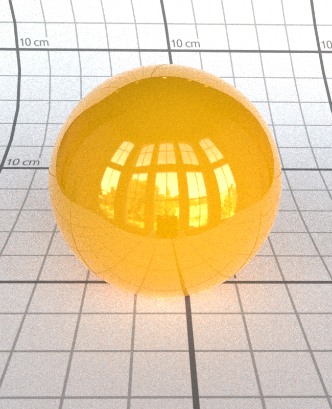
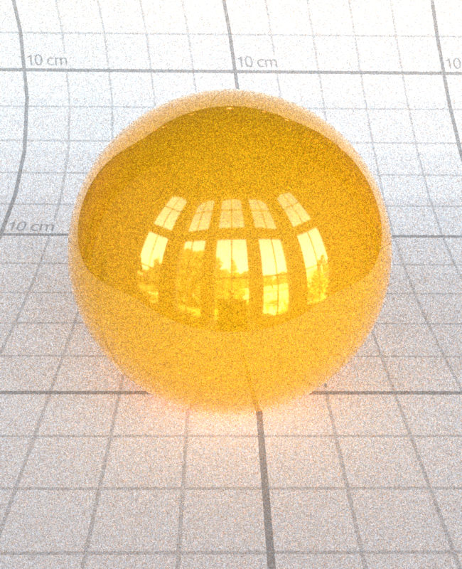
Validation:
All following images are the results from rendering analytical spheres with an
EnvMap Emitter on both Nori and Mitsuba. Note that Mitsuba
takes in a weird transformation matrix for the environment map, so there is
a slight difference of the angle below. The code
for these scenes can be found in scenes/val/envmap/*.xml
and scenes/mitsuba/envmap/*.xml
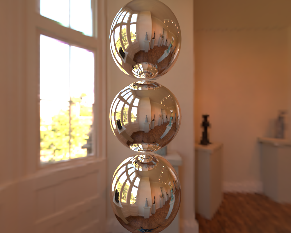

Stacked Spheres with Mirror BSDF

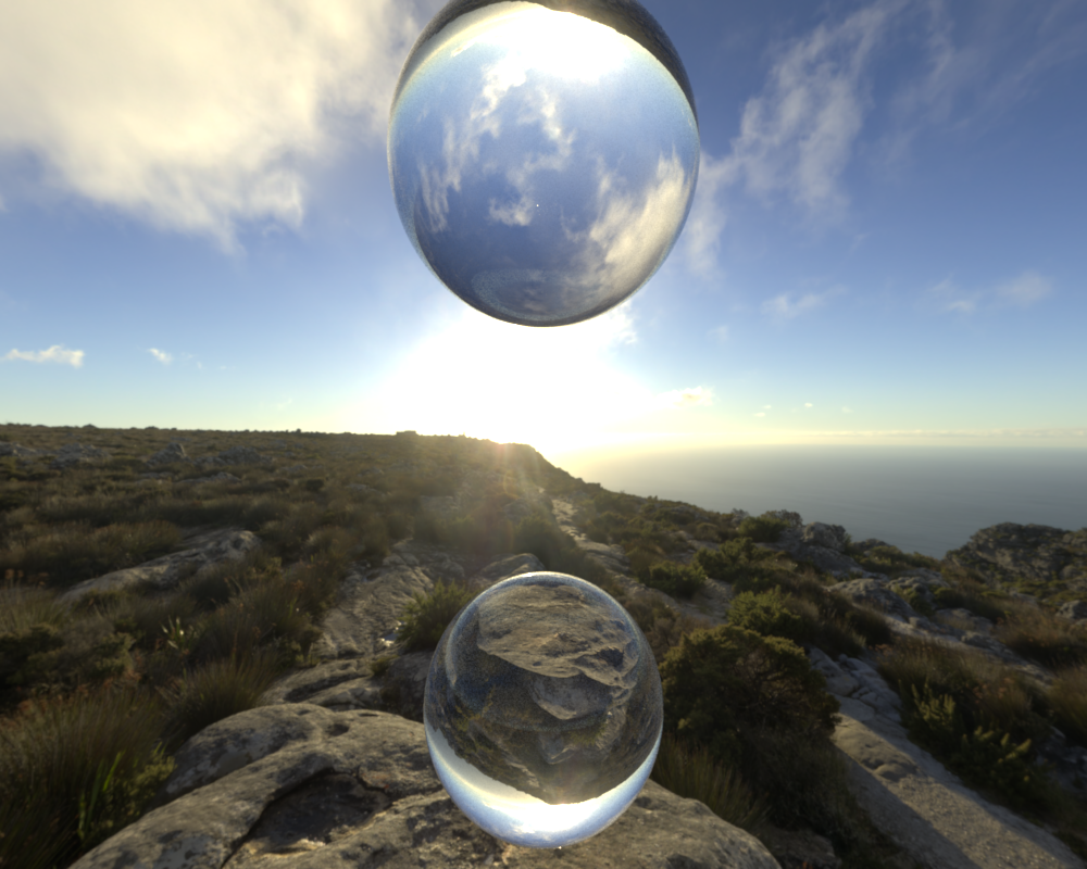
Spheres with Dielectric BSDF
Problems and External Libraries:
Overall, this was one of the more complicated features to implement and hence took more time.
I begin by reading the
PBR 12.6
section on Infinite Area Lights, and explored their implementation. I found myself still stuck
and confused and did quite a bit of research on other sampling methods and explanations of the subject.
I eventually found the paper
Monte Carlo Rendering with Natural Illumination
with a strong description and
pseudocode for a new importance sampling method, and after trying it out it seemed to work well.
There are no external libraries required, and the only thing extra I added was Bilinear Interpolation
for the evaluation. This was probably my favorite feature to implement, and produced a very versatile
way to add backgrounds and lighting to the scene. See src/envmap.cpp for a more
comprehensive explanation of the implementation.